How to use a VLOOKUP Formula

How to use a VLOOKUP formula in Excel with an example

Do you need Microsoft Excel VLOOKUP help or want to know how to VLOOKUP from scratch?

A VLOOKUP function is a great way of collating information, for example if you have someone’s name and address in one worksheet, and their name and phone number in another, you might want to collate their name, address and phone number all in one spreadsheet. A VLOOKUP will enable you to do that.

A VLOOKUP is often used in conjunction with other formulas, such as TRIM, IFERROR and IF(ISERROR) but for now let’s start with a simple VLOOKUP to start with.

To use a VLOOKUP, you need a unique identifier in both sets of data, it could be name, employee ID, product code or anything else unique. A unique number is better than using a name as the unique identifier has to be exactly the same in both sets of data, eg if someone is called Abby in one spreadsheet and Abigail in the other, the formula will not work.

For Microsoft Excel VLOOKUP help, here is an example which can assist your understanding:

The cell which has a unique ID in it is A2 and you are looking at data is in columns G to I

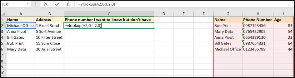
The formula would be = VLOOKUP (A2, G:I, 2, 0) but let’s go through that in more detail:

• Start with Equals (EVERY formula starts with equals!)

• Then write VLOOKUP

• Open brackets

• The cell with the unique identifier e.g. A2

• Comma

• Then the data which has the additional information in it e.g. in this case columns G to I, so select those columns G:I

• Comma

• The number of the column you want to know e.g. if the phone number if what you want to know, and that is in the second column of the data, then it is 2

• Comma

• 0 – technically you should write True or False, and you always write false, but its quicker to just type a zero!

• Close brackets

Warnings
• The unique identifier has to be in the first column of the data you are referring to – eg in the example above, Name is in G and phone number is in H, if name was in H, and phone number was in G, the formula wouldn’t work.

• In the above example, to make it simple, the data was all in one spreadsheet, just some information on the left and some on the right. In practice its more likely the data is in another worksheet, if that’s the case, then you follow the same steps. If the data was in G:I in a sheet called data, the formula would slightly change to =VLOOKUP (A2, Data!G:I, 2 ,0 )

• The main reason why VLOOKUPS have issues, is not the formula, but the data, you need to be 100% sure that the unique identifier is 100% the same in both, that includes no extra spaces which you might not easily see on the screen but are there.

For Microsoft Excel VLOOKUP help, then click here to contact us.
Unlike most Excel spreadsheet training courses - we will not be provide generic Excel spreadsheet training instead each course will be tailored to needs of the group - with the agenda set by the people attending the course.
This training is suitable for employees from all departments and levels of experience.
Training for PCs or Macs.
In London or globally via Zoom to Teams.